Image segmentation plays a crucial role in accurately identifying and delineating objects of interest within an image. In autonomous driving, computer vision algorithms are applied to solve the task of road surface segmentation. This task is challenging as you cannot rely on one type of images only — both cameras and LiDARs have their strengths and flaws. For example, LiDARs provide accurate depth information, but they typically generate sparse point clouds, so they cannot precisely segment objects within the scene. And they may produce distorted clouds when they face transparent or reflective surfaces. Cameras don’t capture the depth, but they provide complete information about the shape, texture, and color of objects. This leads us to a simple idea that an effective fusion of point clouds and images in training 2D road segmentation may harness the advantages of each data domain. The problem is such fusion requires labor-intensive annotation of both datasets. So, can we make data annotation more efficient to enjoy the benefits of a multi-sensor setup for road segmentation?
I currently work at Evocargo. This company provides cargo transportation service and manufactures its own autonomous electric vehicles. As a deep learning engineer, I specialise in the development of 3D detection systems for the autopilot of self-driving vehicles. So, at Evocargo, we decided to find a way to improve the efficiency of road surface segmentation that would keep prediction quality high and reduce annotation costs. After some time of researching and experimenting, my colleagues and I created ==an approach that effectively leverages lidar annotations to train image segmentation models directly on RGB images==. Thus, lidar points projected onto the image and used in further training as ground truth masks provide comparable quality of image segmentation and allow training of models without standard annotated 2D masks.

In this post, I’ll describe our approach step-by-step and show some test results. If you want to dive deeper in our work, other methods research and our test results, then refer to our article ‘Lidar Annotation Is All You Need’ in the IEEE Access journal. This article is supported by the published GitHub repository with the method implementation, processed datasets, and code base for future research. If you find our work useful for your research, please consider giving it a star ⭐ and citing the paper.
Training segmentation models in 4 steps
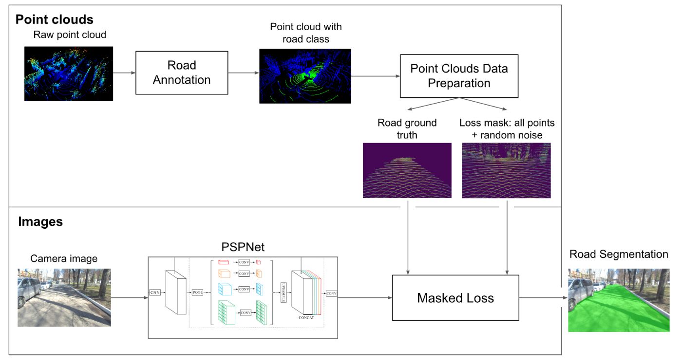
The overall pipeline of our approach consists of four main parts: point cloud road annotation, data preparation, masked loss, and the segmentation model itself.

Firstly, we get the data with road annotations in the point cloud domain. After that, we project points using homogeneous transformations and camera parameters. Then, using the projected points we get the road ground truth mask for loss calculation with added random noise. Images from the camera are processed by the segmentation model. Predictions and masks from the previous step are utilised by the Masked loss, which allows training the model using sparse ground truth data. Finally, after model training, we get an image with a segmented road. The training procedure as well as the Masked loss allow mixing projected ground truth with traditional 2D masks, which makes the approach flexible in terms of data.
Now let’s look closely at each of the parts.
1 Point cloud data annotation
To use lidar data during training, we need semantic segmentation annotations for point clouds. This could be done either manually using an open source point cloud annotation tool, such as Semantic Segmentation Editor, or using some algorithmic approaches. My colleague has described one such approach to road surface detection in his step-by-step guide How to annotate 100 lidar scans in 1 hour. An algorithmic approach especially for road annotation could allow getting without manual annotation at all, but it needs fine tuning for specific data. At Evocargo we use both approaches. For simple areas, the road is annotated algorithmically, and for complex sections – manually.
2 Data preparation
An obtained point cloud is projected on the image plane using homogeneous transformations to get an image segmentation mask with the class label we require, in our case it is a road. For such projection, we use synchronised camera and lidar frames, accompanied by camera parameters, and a transformation matrix from lidar to camera frame. To project homogeneous point x = (x, y, z, 1)ᵀ in lidar frame coordinates to point y = (u, v, 1)ᵀ on an image plane, we use the equation:

After transformation, we get points on the image as a mask of pixels, both for road class and for all other points from the lidar scan. We need other lidar scan points, because the lidar points are mostly located at the bottom of the image and the top of the image has no points at all potentially leading to inaccurate predictions in that area. To eliminate this effect, we add random points in the upper half of the mask (negative class) to balance the distribution of the points where we will calculate the loss.

3 Masked loss
A crucial component of our method is the application of a masked loss function during model training. This approach eliminates the inherent sparsity in lidar-derived ground-truth masks. Unlike conventional loss functions, which consider the entire image masks to calculate errors, masked loss focuses solely on the regions where lidar points are present. This targeted loss calculation ensures that the model’s learning is concentrated on relevant regions, leveraging the information provided by lidar to enhance road segmentation accuracy. In other words, we force the model to learn road segmentation by measuring the error of predictions on a grid of points. It could be compared to looking at the image using shutter glasses (shutter shades).

Masked loss for each image can be formulated this way:

Masked loss is performed by applying a binary mask to the training images. This mask outlines the areas where the lidar points are located and projected onto the image plane. During the training phase, the loss is calculated only for those pixels that are under the mask, effectively ignoring large unannotated parts of the image. This method not only improves the efficiency of the training process, but also mitigates the problems represented by the sparse nature of lidar data.
4 Model training
The final step involves training the segmentation model on the created dataset. The training process can be suitable for any segmentation model, and in our research we used PSPNet. At this stage, everything depends on the quality of your data, its quantity and available computing power.
Promising test results
We tested our approach on various datasets including open-source ones, such as Perception Waymo Open Dataset and KITTI-360 dataset. Each time we conducted a set of three experiments: using only 2D road ground truth, only projected points as ground truth, and a mix of these types of ground truth. And the road segmentation (% of IoU) results look promising:
| Experiment | Trained on KITTI-360 dataset | Trained on Waymo dataset |
|—-|—-|—-|
| 2D only (baseline) | 92.3 | 96.1 |
| Projected 3D only | 89.6 | 94.7 |
| mix 2D + projected 3D | 92.7 | 96.3 |
These numbers mean that if you only have lidar segmentation and do not want to spend additional resources on 2D image annotations, it’s okay. The drop in quality compared to training only on 2D image masks may be insignificant. If you have resources to annotate data from both sensors, then simply combine these two types of annotations during the training process and get an increase in metrics.
All-in-all ==the benefits of the approach== that we observed during the research are:
- high-quality performance of neural networks in image segmentation tasks,
- fewer resources required to annotate data from several types of sensors,
- flexibility to adapt to different image types and segmentation tasks.

Authors of the approach

